
Performance is one of the most common and important metrics of any serious application, and Python code bases are no exception. Performance directly affects user experience and maintenance costs, influencing revenue. Testing and profiling Python code before deployment helps to reveal obvious flaws, whereas investigating incidents after they happen is just firefighting. But how can we dynamically track changes in the application state in production?
The answer is continuous profiling, which lets you discover bottlenecks before they become a problem for the end user.
In this post, we’ll look at Granulate’s continuous profiler, a tool which specializes in continuous profiling and supports practically all programming languages and runtimes—not just Python. Let’s explore how to profile Python code on a Python application example.
Python Application Example
Python Setup With Granulate’s Continuous Profiler
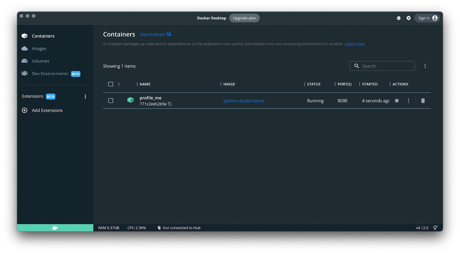
As an example, we’ll use a Python web application, built with Flask and running in Docker. It’s very simple and utilizes only one container:
Let’s start profiling. For that, open Granulate’s profiler, and click the “Free Installation” button. This opens a login page, where you can create an account or use other services (like Google or GitHub) for authorization.
After landing on the home page, click on the “Install Service” button in the right pane to reveal all available integration options, including the one we need—Docker.
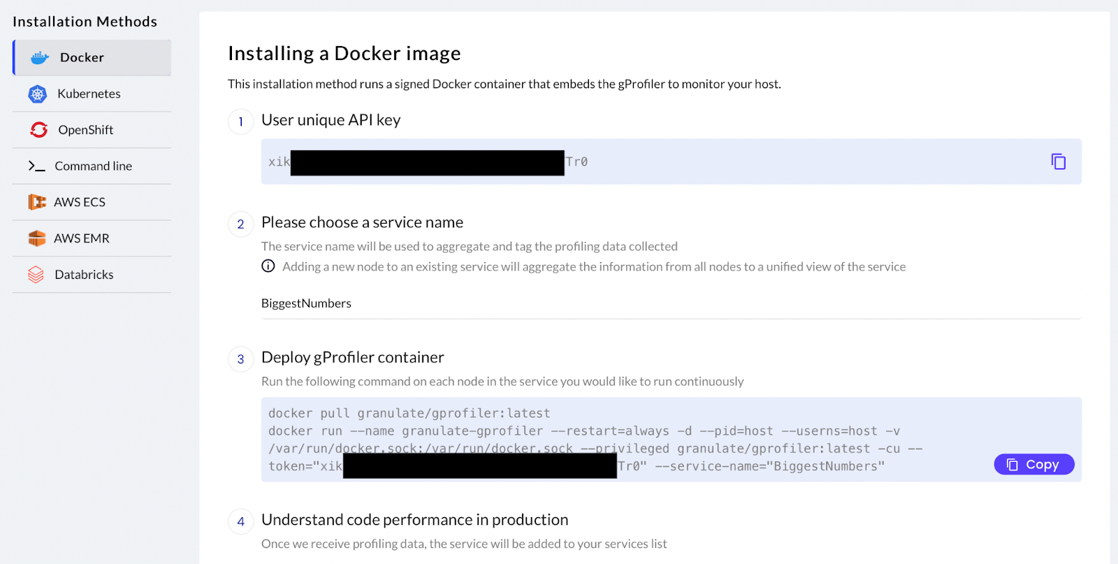
After opening the instructions for Docker, you can see your API key; this is used to configure the profiler, but don’t worry about this. All you need is to pick a name for the service you want to profile (“BiggestNumbers” on the screenshot below).
When the name is entered, two simple commands are generated, which you need to run from the machine or node where the Docker instance is running:
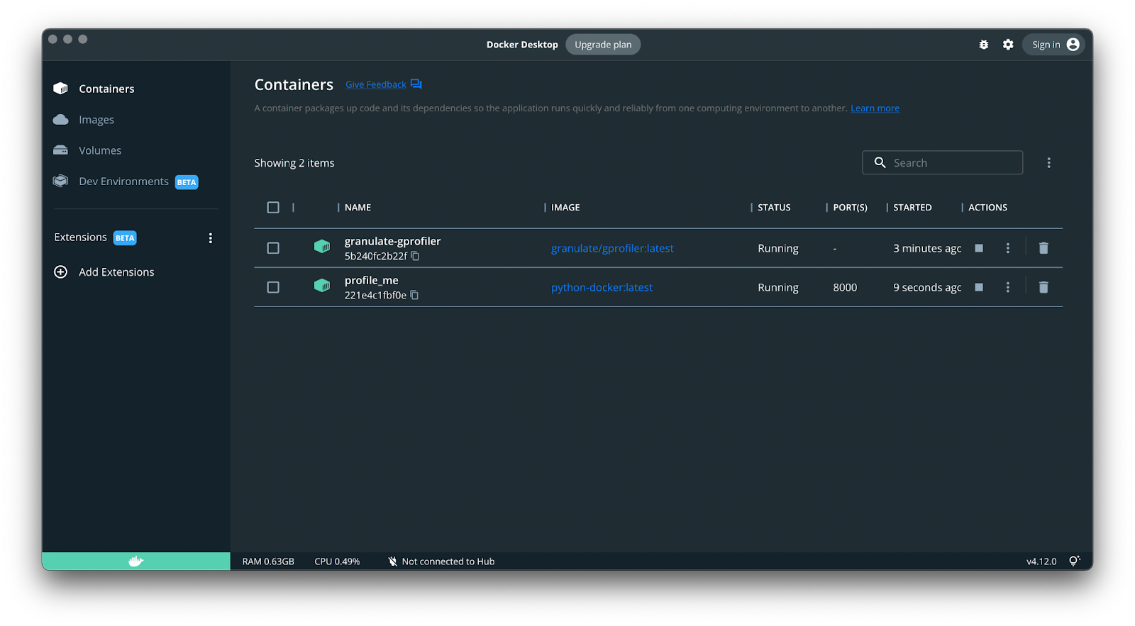
Once that’s done, you’ll see a new container in Docker, which means you did everything correctly:
That’s it! The profiler is configured and ready to use.
Python Usage With the Profiler
Now you can open the Profiles tab in the web interface. After just a couple of minutes, you should see the application there in the drop-down list in the top-left corner of the page.
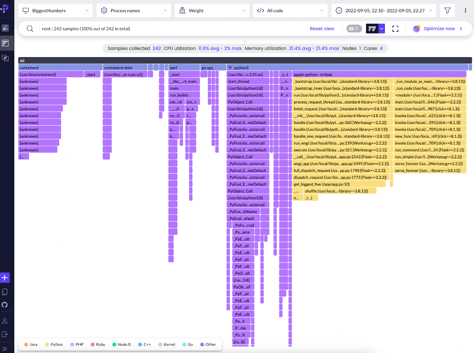
After just a few minutes, the first profiling data should be displayed:

What you see here is called a flame graph. This is the main representation of data we typically use when profiling. While our program is running, the profiler takes snapshots of the system state (CPU and memory usage, functions, call stacks) and sends the data to the server, which then processes the received data and combines the snapshots into graphs.
In the top part of the screen, you can pick a time period to display, and it will show you combined results for that period. The width of the graph indicates the CPU time for the selected period. Each block’s width represents the part of that time that was spent on the corresponding function. Vertically, block chains represent call stacks.
Identifying Python Issues With Continuous Profiling
In the bottom part of a flame graph there is a key that associates the colors of the blocks with programming languages. In our case, we’re interested in the yellow blocks that correspond to Python code. If you look closely, you’ll notice that horizontally, the yellow blocks are the widest and take up more than half of the view—this means it consumes more CPU than anything else in the environment. Hovering over the suspicious blocks will reveal the actual percentage of CPU time that the blocks took and confirm our hypothesis.
We also notice that one of the Python stacks ends with a function called __get_biggest_five_of. Let’s check out its implementation and maybe find the problem:
def __get_biggest_five_of(
numbers_list: List[int]) -> List[int]:
biggest_five = []
while len(biggest_five) < 5:
cur_max = max(numbers_list)
biggest_five.append(cur_max)
numbers_list.remove(cur_max)
return biggest_five
The code looks like a naïve implementation of an algorithm that finds and returns the five biggest numbers in a list of integers. Let’s change the implementation to a call to the heapq method nlargest, which should be more efficient:
def __get_biggest_five_of(
numbers_list: List[int]) -> List[int]:
return heapq.nlargest(5, numbers_list)
Now, re-deploy the program with this change and take a look at the results in the profiler.
After new data arrives and is processed, at first glance, it seems nothing’s different. If you don’t change the displayed time period, the flame graph contains the previous data, and you’ll see a combination of the old and new call stacks:

Again, if you take a closer look at the graph (click on any block to see specific parts of it), you’ll see that the method __get_biggest_five_of is present twice. One of the corresponding blocks is drastically narrower. Let’s hope it’s our fixed version.
To check this, pick a shorter and later period of time, the period after the change came into force. Now, you can observe that the Python code indeed became three times as narrow. If you hover above the method name, it will reveal real numbers of CPU consumption: The new version takes about 60% less CPU time:

Congratulations, you’ve just made your first performance optimization of a Python program, running in a Docker container! The example is, of course, very simplistic. In real-life scenarios, we usually deal with much more complicated and less obvious cases. Still, in these situations, continuous profiling is all the more important.
Granulate Continuous Profiling Capabilities
We’ve gone through a basic example of how you can use the profiler. It’s absolutely free, open-source (unlike most other tools on the market), and extremely easy to install and start using. Also, its user interface is intuitive and flexible, letting you select different time periods, filter processes, etc.
One of the main qualities of the profiler’s UI is that it shows a unified view of your entire system, not just isolated areas, written in a specific programming language.
Additionally, it lets you share graphs and profiled data with other team members by inviting them to the profile, or by exporting it as an SVG image.
Note, the flame graph we used is a key view, but not the only one.
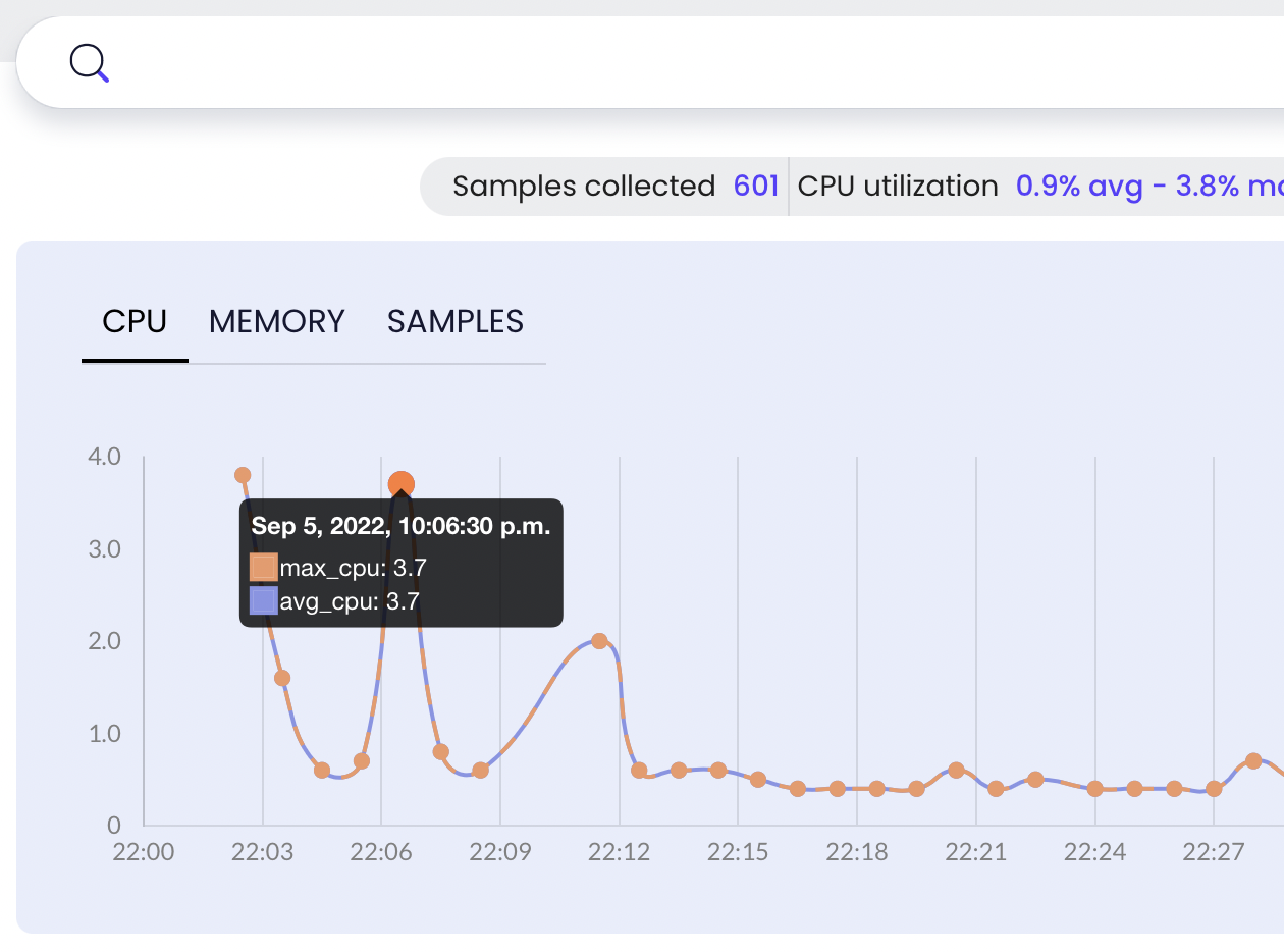
The continuous profiler tracks CPU and memory utilization as well, displaying them in nice charts (see below) for easy viewing. From there, you can monitor for occasional spikes or observe a moment in time when a known performance drop occurred. A great feature of the interface is that it allows you to select a problematic area on a chart and switch to the flame graph, from where you can identify the root cause of the issue:
This profiler is not limited to profiling Python in Docker containers; it supports all programming languages and runtimes, as well as systems, like Kubernetes and Amazon Elastic Container Service. The profiler smoothly integrates into a system for greater observability using an aerial view, or you can drill down for granular detail. Additionally, it uses the eBPF technology to minimize overhead (boasting a utilization penalty of less than 1%) and make data transferring safer.
Conclusion
In this article, we looked at how continuous profiling of a Python application example, running in Docker, can be organized, its benefits, and practical applications. A tool like this can ease the task tremendously. Its friendly and flexible user interface, integration simplicity, and low overhead make the process of profiling a breeze.
As mentioned, some other profilers offer similar features but come with their own limitations and are mostly paid and, alas, never open-source.
So take an interactive tour of Granulate’s profiler today, and see how your production profiling can be made easy.