

CPU profiling is not a new concept and has been around for decades. However, with advancements in profiling techniques and a push towards observability, profiling is today seeing a steady rise in adoption.
Profiling helps you understand code-level performance and optimize the resource-consuming parts of your code. You can also profile your application to perform root-cause analysis.
Traditionally, since profiling introduced a lot of overhead to be run on production systems, it was more of an ad-hoc process, only done for root cause analysis and to look for specific issues. But with the advent of eBPF-based profiling, continuous profiling of your applications is now possible with very low overhead.
Intel Tiber App-Level Optimization has one such continuous profiling tool that you can incorporate into your stack to reap the benefits of continuous profiling and proactively look for optimization opportunities.
In this post, we’ll see how to use continuous profiling on your entire server including both the user and kernel stack.
Setup
We’ll be using Docker Compose to set up the profiler agent on our server. The subsequent section has detailed steps to run the profiler agent via Docker compose. But before getting started, you’re gonna need an account (which is free).
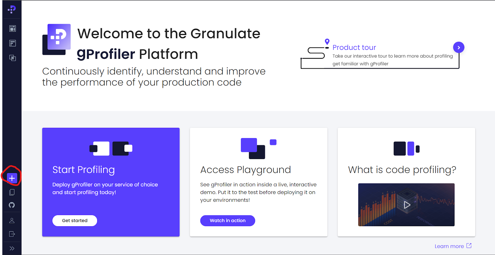
So, go to https://profiler.granulate.io/ and sign up for an account. Once done, click the “+” sign and choose the installation method as Docker.
You’ll see your unique User API Key and steps to run the profiler Docker container. The agent will pass this API key as a token to authenticate to Intel Tiber App-Level Optimization’s backend. Just Enter the Service Name as “gprofiler-demo,” and you’ll see the Docker run command being generated for you.

Since we’re using docker-compose, we won’t need this Docker command, but if you want to run the container directly, you can copy-paste it and run the container.
We will use the sample docker-compose file to run the profiler agent, so save the template as a docker-compose.yml file.
Next, replace the token and service-name parameter according to the previous step, then run the agent with the following command:
docker-compose -f docker-compose.yml up -d
You should see the following output:
Starting granulate-gprofiler … done
You can also confirm if the agent is running by issuing a docker ps command, after which you should see a container running.
Now, go to your dashboard and navigate to the Profiles tab, where you should see a flame graph for your server.

Figure 3: Flame graph after installing running profiler agent
A few things to note on the screen:
- The name of your service that you configured, in our case, gprofiler-demo
- The overall stats of your server, CPU, and Memory utilization
- The flame graph itself
Note: Your flame graph might look different based on the processes you have running on your machine.
Next, click on the Process Names drop-down to see all the processes running.

Currently, the only applications running on our server are the Docker engine (containerd), Docker Compose, our profiler agent container, and associated profiler.
But let’s now zoom in a bit on our flame graph.

You can see there’s a flame for each of our processes. The width of the flame shows the amount of CPU time being used by that process. The python3 process is the widest of all, which means it’s consuming the most CPU at the moment.
Each frame represents a function call, while the different colors denote the different languages of each call frame. Yellow is for python calls and pink for kernel calls.
Now, hover over the widest flame, python3.
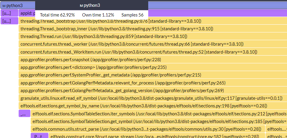
You’ll note three stats being shown. You can hover over any frame, and you’ll see the same three stats:
- Total time: Percentage of CPU time consumed for all the frames below the frame you are currently hovered over, 62.92% in our example above
- Own time: Percentage of the total time the current frame is consuming, here, 1.12%
- Samples: Number of samples collected for this flame and stats to be generated
We can inspect even more frames below this.
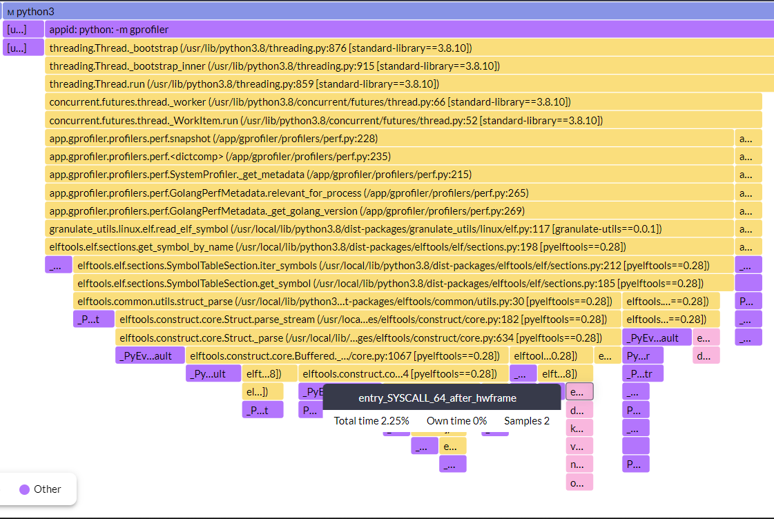
This kernel frame (and the frames under it) is consuming 2.25% of the total 62.92%. But the current frame is consuming 0% (Own time). So, which frame is consuming the time? Let’s find out.

Turns out, the last frame (which is a kernel frame) is the one consuming 2.25% of the CPU time.
That’s how you can drill down for each process and see which frame is consuming the most CPU time. If this was a real application, the frame hogging the most CPU time would be a good candidate for optimization. Conversely, if you were seeing bad performance in your application, you would look for the widest frame in your app’s flame graph to find the one causing bad performance.
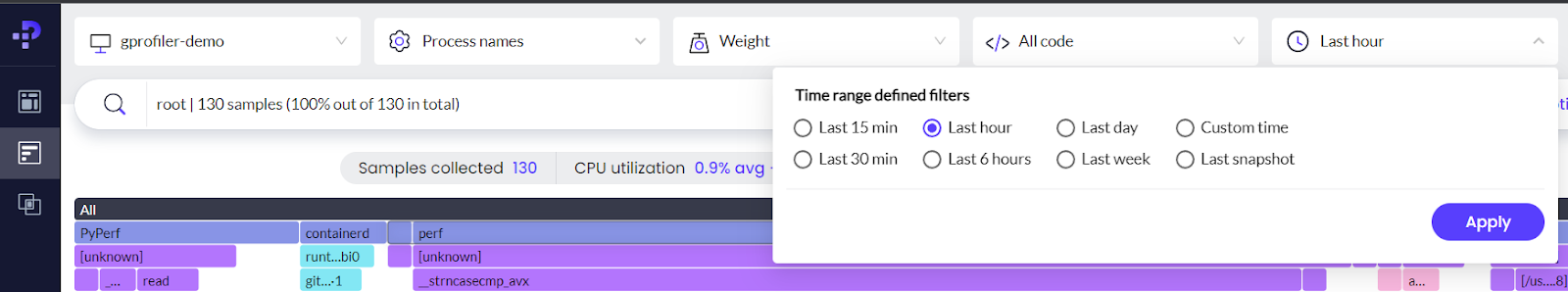
The profiler lets you change the time range for which you can analyze the graph.
The dashboard also has a table view, which shows the information in tabular form if that’s easier for you to understand. Just use the Table View button to switch.
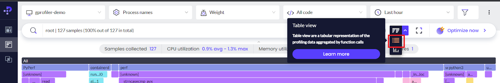
You can also see stats in tabular form for each stack you saw in the flame graph.

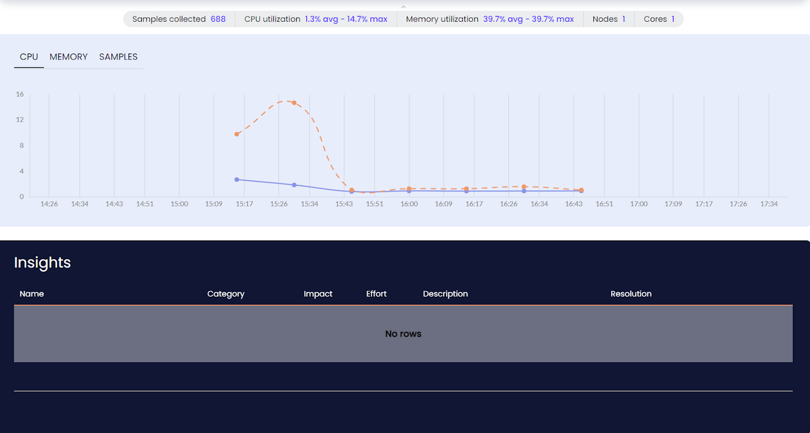
We can even filter this view for a particular process or time frame. Meanwhile, Service Overview gives you details of CPU and Memory usage over time.
Before we move on to deploy a sample Scala application and see how flame graphs can help us find poorly performing code, let’s take a look at some of the salient features of Intel Tiber App-Level Optimization’s continuous profiler based on our demo so far.
- It has a very low memory and CPU footprint. The average CPU utilization is less than 1% if only the profiler is running.
- It supports system-wide profiling, giving you insights into all the programs running on your machine.
- Our example uses Docker, but it also supports Kubernetes, Dataflow, Spark, and many other distributed systems, taking your observability to the next level.
- Lastly, there’s ease of deployment. We just had to run one Docker container and pass it our API key, and within a few seconds, we could see our flame graphs and server stats.
In the next section, we’ll deploy a Scala application with a CPU-hogging regex; we’ll then analyze the flame graph and find out which frame is causing the issue.
Scala Application Example
So, we have a small program that searches for a regex pattern in a large corpus of text. The issue with the application is that the search function is hogging a lot of CPU and performing badly. We’ll analyze the app’s flame graph and try to figure out which part is actually taking up CPU; then, after finding and fixing the problem, we’ll see how our flame graph changes.
So let’s get started.
We have a small snippet of Scala code that basically applies a regex filter to a large string corpus. In this example, we’re using the entire text of Shakespeare’s Hamlet from here. Then, we’re gonna try to search the string HAMLET in the entire corpus and print the number of matches a million times.
Once we run the code below, we’ll see the flame graph for it:
object App {
def main(args: Array[String]): Unit = {
for(i <- Range(1,1000000)) {
val corpus = Source.fromResource(“corpus.txt”).getLines().toList
println(s”Total lines ${ corpus.size }”)
val matches = search(corpus, “[h|H][a|A][m|M][l|L][e|E][t|T]”)
println(s”Total Matches ${ matches.size }”)
}
}
def search(corpus: List[String], pattern: String): Seq[String] = {
corpus
.flatMap(line => line.split(“s+”)) // Split Words
.filter {
case word =>
val regex = new Regex(pattern)
regex.matches(word)
}
}
}

From the flame graph generated, we can see that the majority of the width (hence CPU) is being used by our program. You can even check the Service Overview chart and see that 100% of the CPU is being used.

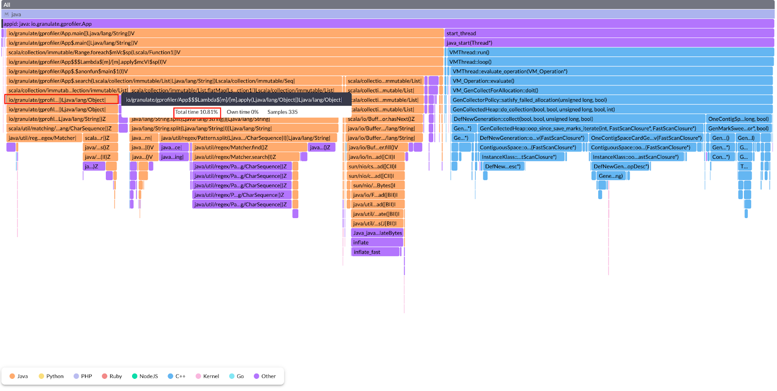
Let’s zoom in on our process now. Click on the stack of our app to zoom into the flame graph of just our application.
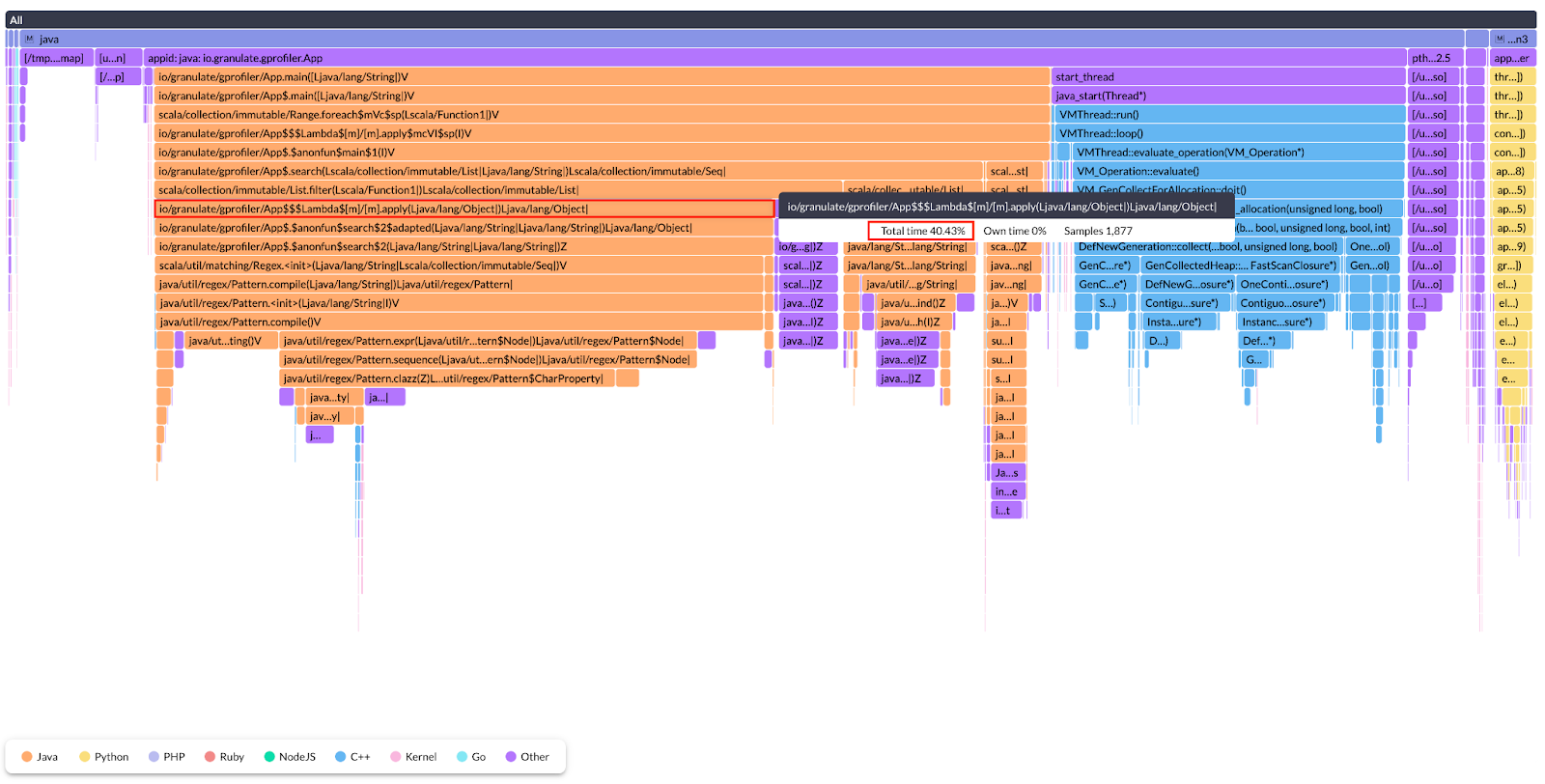
You can see that the majority of the CPU is spent executing our Scala code. Also, if you look further, you’ll find that our lambda expression for filtering is taking a good chunk of CPU (~40% of total process time), which should not be the case.
Let’s see if our code can tell us why this is happening. Upon closer inspection, you’ll see that we made a mistake in our code. We’re compiling a regex pattern inside the loop, which means the pattern will get compiled in every iteration.
Let’s move it outside the loop block and rerun the code to see if anything changes:
object App {
def main(args: Array[String]): Unit = {
for(i <- Range(1,1000000)) {
val corpus = Source.fromResource(“corpus.txt”).getLines().toList
println(s”Total lines ${ corpus.size }”)
val matches = search(corpus, “[h|H][a|A][m|M][l|L][e|E][t|T]”)
println(s”Total Matches ${ matches.size }”)
}
}
def search(corpus: List[String], pattern: String): Seq[String] = {
val regex = new Regex(pattern)
corpus
.flatMap(line => line.split(“s+”)) // Split Words
.filter {
case word =>
regex.matches(word)
}
}
}
After moving the regex creation out of the loop, you can see that the CPU utilization has dropped significantly. And the width of the flame is now significantly smaller than the previous version.
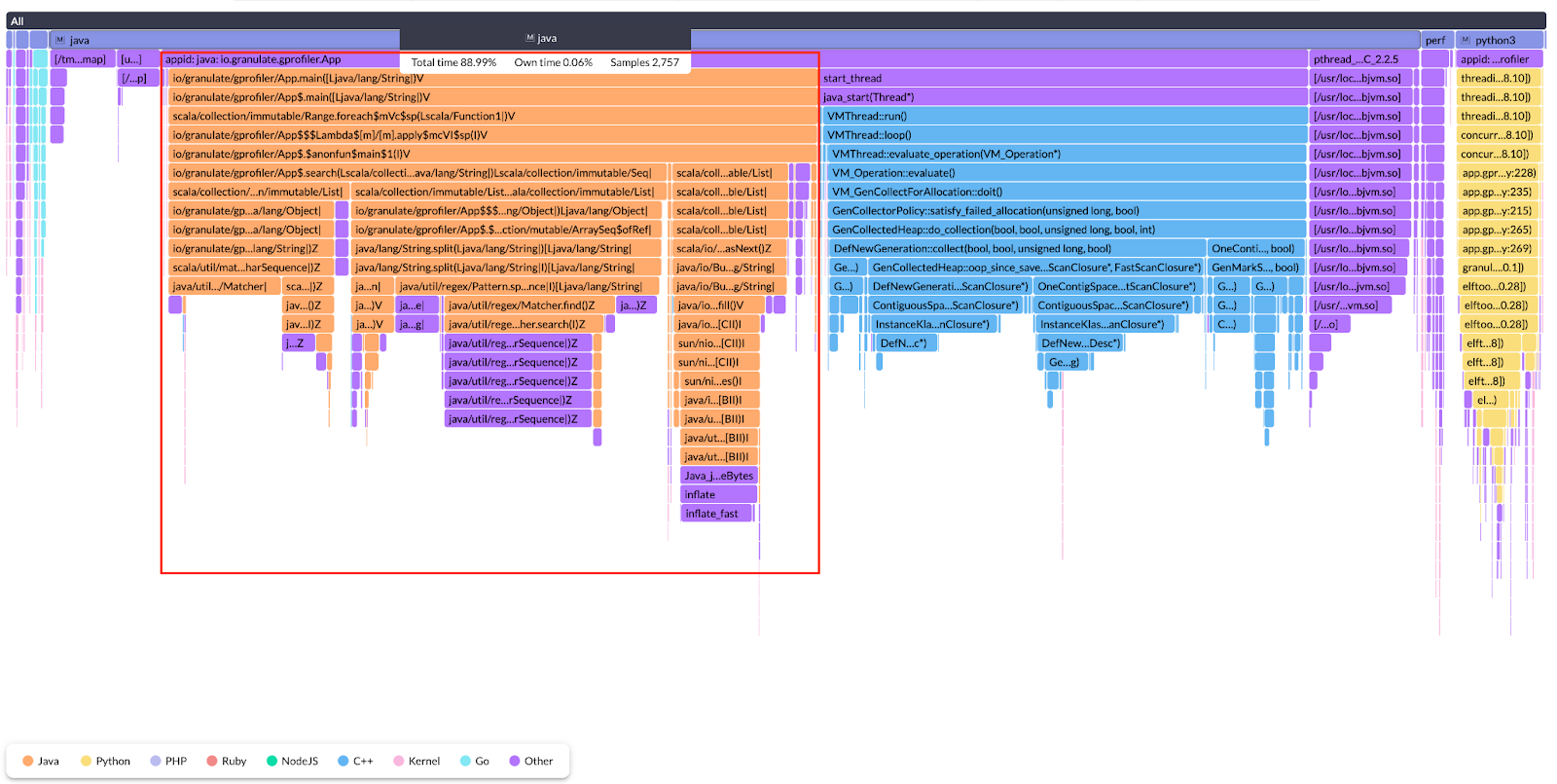
Zooming even more into the flame, you’ll see that the flame for the execution of our loop has also gone down in width. And the giant lambda expression stack is narrower now, pointing to the fact that moving the command out of the loop has improved overall CPU utilization. In the optimized code, the lambda expression is consuming only ~10% of CPU time as opposed to ~40% in the unoptimized version.
This is how we can use flame graphs to identify bottlenecks and pinpoint the places in our code causing those bottlenecks.
You can also share the flame graph with other team members by clicking on the three dots in the top right corner. Moreover, you can download the flame graph in SVG format to share via email or message apps (e.g., Slack, Teams).

Conclusion
To recap, we’ve learned how Intel Tiber App-Level Optimization’s continuous profiler uses sophisticated techniques like eBPF to achieve low-impact continuous profiling. We also saw how continuous profiling is actually better for production systems, as it allows you to proactively discover places for optimization in your applications before they start impacting your end users. We learned how to read flame graphs and interpret them to figure out hotspots in your applications. In the example we used the flamegraph to find the issue in the code and fixed it to reduce ~30% CPU utilization. Lastly, we saw how you can invite other team members to access the profiler dashboard in real time or simply share exported flame graphs.
Having a continuous profiler in your observability stack can really help you proactively optimize your application, which in turn elevates the user experience and overall resource utilization.