
Congestion control in network layer occurs when a node or link carries data beyond its limit. This often leads to the queuing of packets—and in the worst case, loss of packets—as well as a decrease in the network’s Quality of Service (QoS).
Sudden bursts of traffic due to special events can also choke otherwise healthy and sufficient network links resulting in a degradation of the entire network. Yet another cause of network congestion is network protocols that use retransmission to avoid packet loss, such as TCP (Transmission Control Protocol, the backbone of the modern internet), which can keep a network congested even when the load has been reduced. Such a state where the initial load has died down but network throughput is still low is called Congestive Collapse.
In this post, we will discuss how to achieve congestion control in network layer via various algorithms and avoid congestive collapse.
What Is Congestion Control?
A network is a shared entity used by multiple parties in a collaborative manner. However, a few faulty or unverified network users (data senders) can cause congestive collapse where the Quality of Service is so degraded that it prevents or limits any useful communication.
Congestion Control is a mechanism that controls the entry of data packets into the network, enabling a better use of a shared network infrastructure and avoiding congestive collapse. Congestive-Avoidance Algorithms (CAA) are implemented at the TCP layer as the mechanism to avoid congestive collapse in a network.
Congestion-Avoidance Algorithms
In layman’s terms, congestion-avoidance algorithms work by detecting congestion (through some sophisticated mechanisms we’ll cover later on) and adjusting the data transmission rate to avoid it. This ensures the network is usable by everyone.
Congestion control occurs at different parts of the network, from Active Queue Management that reorders packets in the Network Interface Controller (NIC) to variations of Random Early Detection in routers.
Since the backbone of the entire internet is based on Layer 4 Transmission Control Protocol, this article will cover concepts and algorithms from the standpoint of TCP.
But before we delve deeper into different algorithms, let’s first learn some terminology:
TCP Glossary
Maximum Segment Size (MSS): A property of the TCP layer, MSS is the maximum size of a payload that can be sent in a single data packet. This size does not include the header size.
Maximum Transmission Unit (MTU): The maximum size of a payload including the headers that can be sent in a single packet. This is a property of the Data Link layer. The difference from MSS is that if a packet exceeds MTU, it is broken into multiple chunks obeying the MSS of the link. However, if a packet exceeds the MSS, it is dropped altogether.
Cwnd (Congestion Window): The number of unacknowledged packets (MSS) at any given moment that can be in transit. The congestion window increases, decreases, or stays the same depending on how many of the initial packets were acknowledged and how long it took to do so.
Initcwnd (Initial Congestion Window): The initial value of cwnd. Usually, algorithms start with a small multiple of MSS and increase sharply.
Fast Retransmission: This algorithm improves TCP by not waiting for a timeout for any particular packet to be retransmitted. If the sender receives three duplicate ACKs (additive increases) for a packet (i.e., a total of four ACKs for the same packet), it assumes that the next-higher packet is lost and retransmits it immediately.
Now, let’s see how TCP works and how congestion-avoidance mechanisms kick in.
TCP Connection Lifecycle
When a connection is established, the sender does not immediately overwhelm the network; instead, it starts slow and then adjusts according to the network bandwidth.
In TCP, the congestion-avoidance mechanisms kick in when the network detects loss because TCP perceives every loss as an event due to congestion. There are two ways in which TCP assumes that packets are getting lost:
- When there is a timeout
- When the server receives three duplicate ACKs for a data packet
Different algorithms have different behaviors for both starting out the connection and avoiding congestion.
Below, we’ll discuss two such mechanisms: Additive Increase Multiplicative Decrease and Slow Start.
Additive Increase Multiplicative Decrease (AIMD)
In this approach, senders increase the cwnd by 1 MSS on every successful ACK (additive increase). On the detection of loss, the cwnd is cut in half (multiplicative decrease). This shows a saw-tooth behavior in cwnd.
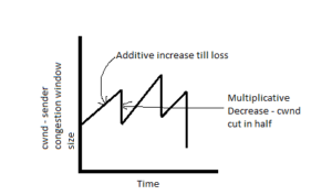
Figure 1: Saw-tooth behavior of cwnd in AIMD algorithm
Slow Start
Contrary to its name, this algorithm starts with initcwnd set to 1 and doubles the cwnd after every successful ACK until it reaches the ssthresh (Slow Start threshold), after which it increases the cwnd linearly by 1 MSS on every ACK.
When a loss is detected, the ssthresh is set to one-half of the cwnd at that time, and cwnd is decreased. (Algorithms can have different ways of decreasing the cwnd, as we will see in the next section.)
Examples of Congestion-Avoidance Algorithms
Over time, a lot of congestion-avoidance algorithms have been introduced in the network stack. In this section, we’ll cover some of the most prominent ones and learn how they compare to one another.
TCP Tahoe
This is an algorithm based on the Slow Start mechanism. It starts in the slow-start phase where the cwnd increases exponentially until cwnd reaches the ssthresh value, after which cwnd increases linearly. When packet loss is detected, Tahoe reduces the cwnd to 1 and ssthresh to half of the current cwnd. Tahoe follows the same congestion-avoidance phase no matter if the loss was because of a timeout or due to duplicate acknowledgments.
TCP Reno
This algorithm is a slight enhancement on Tahoe and behaves differently when packet loss is detected because of duplicate ACKs. In this scenario, the cwnd and ssthresh are both set to half their current value, and instead of proceeding in the slow-start phase again, the cwnd increases linearly.
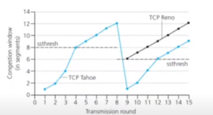
Figure 2: TCP Tahoe vs. TCP Reno: Post-congestion behavior (Source: Anand Seetharam, YouTube)
TCP Westwood+
An improvement over TCP Reno, instead of blindly setting cwnd to half upon receiving three duplicate ACKs, this algorithm adaptively sets both the ssthresh and cwnd based on an estimate of bandwidth available at the time congestion is experienced. Westwood+ optimizes performance over both wired and wireless networks.
CUBIC
This algorithm is an improvement over both Tahoe and Reno. It implements a concept of Hybrid Start (HyStart) instead of the regular Slow Start from TCP Tahoe, Reno, and Westwood+. The standard slow-start approach causes high packet loss during an exponential increase in cwnd and makes it difficult for the network to recover.
In the CUBIC algorithm, following the function below per the official documentation, cwnd is based on the time since the last congestion event occurred and not on how fast ACKs are received:
cwnd = C*(t-K)^3 + W_max
K = cubic_root(W_max*(1-beta_cubic)/C)
Where:
- Beta_cubic is the multiplicative decrease factor.
- W_max is the window size just before the last reduction.
- T is the time elapsed since the last window reduction.
- C is a scaling constant.
- Cwnd is the congestion window at the current time.
This allows HyStart to get out of the slow-start phase quickly and move into the congestion-avoidance phase without much packet loss. According to a comparative study, HyStart improves the startup time of a TCP connection by two to three times.
Bottleneck Bandwidth and Round-Trip Propagation Time (BRR)
This congestion-avoidance algorithm was developed at Google and claims to increase TCP performance by 14%. Contrary to the loss-based algorithms that we have covered so far, BRR is model-based. It creates a model of the network to adjust the transmission rate rather than use a rule-based approach. The model is built with maximum bandwidth and round-trip time at the instant the most recent data packet is delivered.
As networks evolve from megabit to gigabit speeds, latency becomes a better measure for throughput instead of packet loss, making model-based algorithms like BRR a more reliable alternative to loss-based algorithms.
When used by YouTube, traffic saw an average increase in speed of 4%. BRR is also available in Google Cloud Platform.
Currently, there are two versions of BRR available, v1 and v2. BRRv1 is disputed to be unfair for non-BRR datastreams, hence BRRv2 deals with the issue of unfairness by adding information about packet loss to the model.
Current State of CAA in Linux Kernels
Up until 2009, a mix of high-bandwidth, low-latency, and lossy connections were not very common, so CAA algorithms from that era are not suitable for today’s high-latency and lossy mobile connections. However, most Linux boxes today are running a kernel version from pre-2009 (2.6.32.x) and are thus only equipped with outdated CAA algorithms.
But in kernel version 2.6.38, the default value of initcwnd was bumped from 3 to 10, allowing you to send/receive more data in the initial round trip (14.2 KB as opposed to 5.7 KB) and giving you more space to put protocol headers.
Meanwhile, kernel version 3.2 implemented the Proportional Rate Reduction (PRR) algorithm, which resulted in a reduction of recovery time for lossy connections. This had a positive impact on HTTP response times of 3-10%. This version also altered the Initial Retransmission Timeout (initRTO) to 1s from 3s, resulting in the saving of 2s if the packet loss happened after sending the initcwnd.
Irrespective of kernel version, the tcp_slow_start_after_idle setting should be changed to get a significant improvement in network performance. Out of the box, the value is 1, which decreases the congestion window on idle connections, in turn affecting long-lived connections like SSL.
The following command will set it to 0 and significantly improve performance:
sysctl -w tcp_slow_start_after_idle=0
Conclusion
Since the early days of the internet, efforts have been made to create a CAA that helps deliver high throughput and low latency even in the face of mixed networks (wired, mobile, wireless). It wasn’t until the late 2000s that older algorithms started showing their age and the need for more refined algorithms emerged. That’s when kernel developers and large organizations like Microsoft and Google started investing both time and money in developing advanced CAA algorithms.